2048 Game AI
2048 is an online/mobile game which was originally released in 2014. The game begins with two randomly placed tiles, each having a value of either 2 or 4, randomly placed on a 4x4 grid. The player can move the tiles in four directions: up, down, left, or right. When a direction is chosen, all tiles on the grid slide as far as possible in that direction, merging with any adjacent tiles of the same value to form a new tile with double the value. The value of the new tile is added to the score. After the player’s turn, a new tile spawns in a random location; this new tile has a 90% chance of being a 2, and a 10% chance of being a 4. The game ends when the board is filled with tiles and the player has no legal moves. The goal of the game is to combine tiles until the 2048 tile is reached (although it is possible to continue playing after winning).
I first implemented A Pure Monte Carlo Tree Search algorithm, and then improved performance by formalizing the game’s state tree as a Markov Decision Process. The final algorithm I designed achieves the 2048 tile 97% of the time and the 4096 tile 58% of the time.
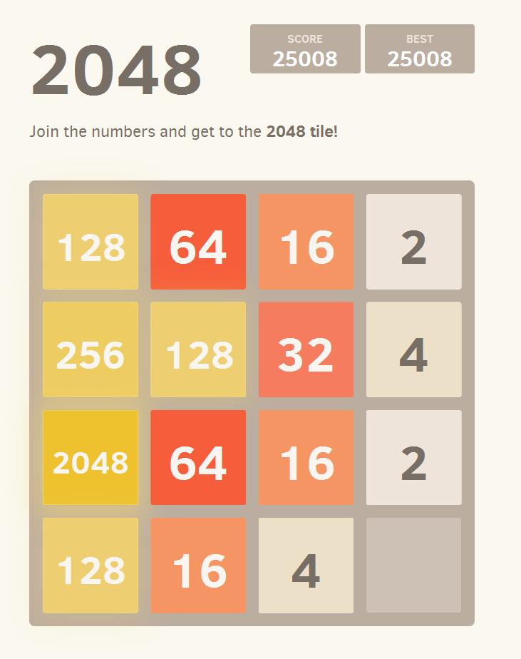
Original Game
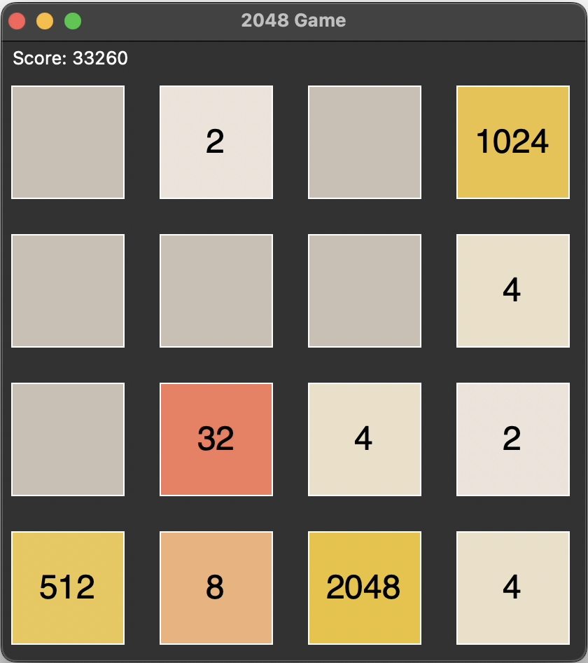
My Python Clone
Screenshots from original game and my implementation
The decision tree
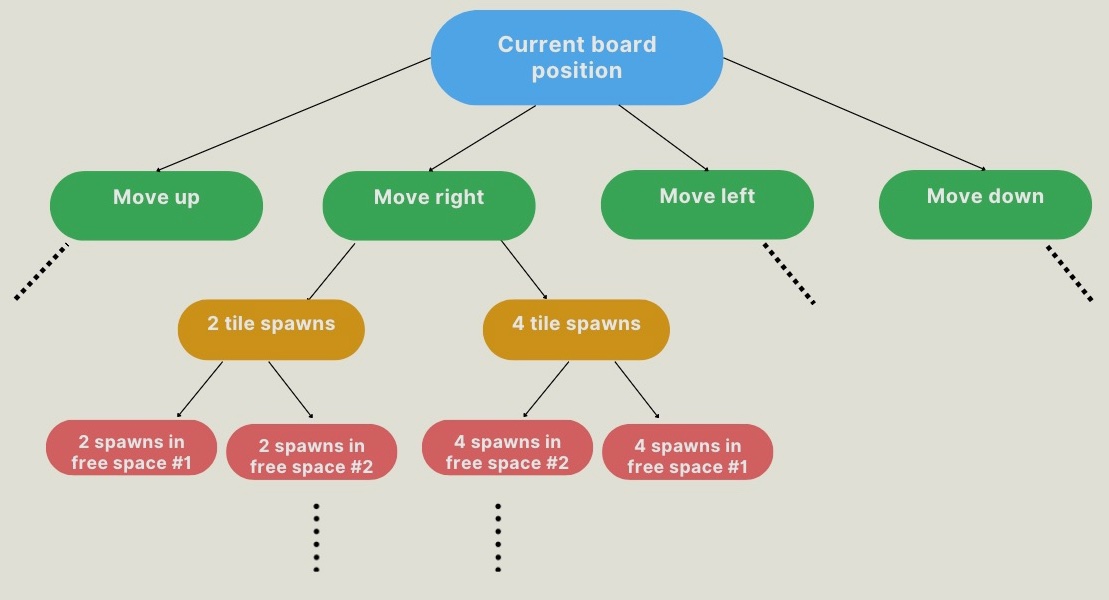
One of the challenges of creating an AI which plays 2048 is the sheer number of possible games. Figure 1 represents the possible board positions after the player makes only one move. If there are 8 free spaces on the board, for example, then there are 64 possible game states after the player’s move (assuming each of left, right, up and down are legal moves which do not combine any tiles). In general, there are 2(|S|)(m) + c possible states after the player’s move, where |S| is the number of legal moves, m is the number of empty spaces on the board after tiles have been combined from the player’s turn, and c is the number of tiles which get merged as a result of the player’s move.
AI designs
The initial algorithm I developed is a simple Pure Monte Carlo Tree Search (Algorithm 1). This algorithm takes the current game position and the desired number of simulations per direction $(n)$ as inputs. It explores all legal next moves from the current position by simulating $n$ games for each potential move. Each of these simulated games is played by making random moves until the game is over. The scores from the end of these simulated games are then averaged to determine the quality of each move. The direction with the highest average score is selected:
This approach initiates from the green nodes in the game tree diagram (Fig. 1). From there, the algorithm proceeds through random exploration to reach the red child nodes, representing the spawning of a 2 or 4 tile in each possible location.
While this approach provides a comprehensive exploration of the game tree, it has significant limitations. The primary concern lies in the random nature of the search process. As a consequence, some of the simulated games performed during the Monte Carlo simulations may yield exceptionally poor results that are highly unlikely to occur in actual gameplay. This lead me to want to discard a portion of those simulated games with particularly poor scores from consideration.
Simply modifying Algorithm 1 to calculate the average score for a given move using only top-performing of simulated games would not adequately address this source of randomness, however. There are two sources of randomness inherent in the Pure Monte Carlo Tree Search: randomness associated with game-play (which I aim to reduce), and randomness of tile spawns. Discarding randomly played games with low scores in an attempt to address the former source of randomness might prevent the AI from evaluating branches of the tree which involve unlucky tiles spawning after the next turn.
\begin{algorithm}
\caption{Pure Monte Carlo Tree Search}
\begin{algorithmic}
\FUNCTION{PMCTS}{currentPosition, n}
    \STATE $directionScores \gets \text{list()}$
    \FORALL{$nextMove \in legalMoves(currentPosition)$}
        \STATE $nextMoveScores \gets \text{list()}$
        \FOR{$gameNumber \gets 1$ \TO $n$}
            \STATE $result \gets playRandomGame(currentPosition, nextMove)$
            \STATE $nextMoveScores.append(result)$
        \ENDFOR
        \STATE $averageScore \gets mean(nextMoveScores)$
        \STATE $directionScores.append(averageScore)$
    \ENDFOR
\RETURN $directionScores$
\ENDFUNCTION
\end{algorithmic}
\end{algorithm}
Markov decision process
Some of the pitfalls of the Pure Monte Carlo Tree Search can be circumvented by formalizing the game structure as a Markov Decision Process (MDP). The core functionality of the MCTS is used as part of the MDP-based strategy, but the evaluations made with MCTS are made more beneficial by explicitly maximizing expected value. Where the PMCTS algorithm begins Monte Carlo simulations from the board state after a player’s move (green nodes in Figure 1), The MDP strategy begins Monte Carlo simulations from each possible tile spawn in response to a player’s move (red nodes in Figure 1). It is possible to model the game as a Markov decision process because the game satisfies the Markov property: the probability of reaching a future state depends only on the current state, not on previous states:
In general, an is MDP is characterized as follows: 1. S: The set of states (board position and score) which could arise after the AI’s next move. 2. A: The set of actions which the AI could legally take from the current position. 3. P(s’|s, a): Transition probability of reaching state s’ given current state s ∈ S after taking action a ∈ A. 4. V(s): The value function which determines the expected future reward associated with entering a state s ∈ S. 5. π(s): The policy function which uses the other functions to strategically pick an action a ∈ A given any board state. 6. R(s): The immediate reward associated with taking action a ∈ A which leads to state s ∈ S is a part of many MDP algorithms.
$A$ can be constructed by checking which of left, right, up or down are legal moves. $S$ can be constructed by placing a 2 and then a 4 on each empty tile for each $a \in A$ (Algorithm 2). The value function, $V(s, \vec{\theta})$, (Algorithm 3) performs a Monte Carlo tree search, with the number of simulations determined by the parameter vector $\vec{\theta}$. $\vec{\theta}$ contains the following parameters:
- Number of random searches for 2 spawning with 1-3 empty tiles.
- Number of random searches for 2 spawning with 4-6 empty tiles.
- Number of random searches for 2 spawning with 7-9 empty tiles.
- Number of random searches for 2 spawning with 10-15 empty tiles.
- How many times more searches 2 spawns should get compared to 4 spawns.
- Top proportion of best performing moves to include for score evaluation.
$\theta_1, \theta_2, \theta_3$ are scaled so their respective empty tile ranges have the same total number of simulations. $\theta_4$ uses the same number of simulations for each of 10-15 empty tiles. If $\theta_1 = 500$, for example, the Monte Carlo simulation will run 500 times when there is one tile, 250 times when there are two, and 125 when there are three; if $\theta_4 = 20$, then the Monte Carlo simulation will run 20 times for any number of empty tiles $\in [10, 15s]$.
$\vec{\theta}$ remains constant throughout a single play-through of the game. The policy function, which determines what action $a \in A$ to take, $\pi(s)$, is given by Equation $\eqref{MC12_policy_fn}$:
Notice that $\pi(s)$ picks the action with the highest expected value, where the value associated with reaching a state is given by a Monte Carlo tree search. Compared to the Pure Monte Carlo Tree Search, the MDP-based algorithm facilitates more sophisticated inference in two ways.
-
By discarding a portion of explored games with poor results at each node, the impact of the Monte Carlo search playing out extremely poor moves due to chance can be mitigated. Crucially, simulations with lower scores due to “unlucky” tile spawns in the subsequent turn are not eliminated, ensuring a more comprehensive exploration of potential game outcomes.
-
Unlike the Pure Monte Carlo Tree Search, where game states in which a 2 spawns after the player’s turn are explored 9x as frequently as those in which a 4 spawns, the number of Monte Carlo searches on each node type can be made independent. This can guarantee that all nodes are explored at least 3 times, which gives information with far lower uncertainty than a node being explored 1 time, while not significantly increasing runtime.
The MDP-based algorithm is implemented in a manner which makes customizable the number of Monte Carlo searches per node $(\theta_1 - \theta_5)$ and proportion of top-performing simulated scores to keep $(\theta_6)$. Each of these parameters impact the reported score associated with a direction, and therefore the move selected by $\pi(s)$.
\begin{algorithm}
\caption{Generation of possible next states}
\begin{algorithmic}
\FUNCTION{GetStates}{A}
    \STATE $S \gets \emptyset$
    \FORALL{$a \in A$}
        \STATE $c_s \gets$ score associated with taking action $a$
        \FORALL{$tileNum \in \{2, 4\}$}
            \FORALL{$tile \in emptyTiles$}
                \STATE place $tileNum$ on $tile$
                \STATE $s \gets (board, c_s)$
                \STATE add $s$ to $S$
                \STATE remove $tileNum$ from $tile$
            \ENDFOR
        \ENDFOR
    \ENDFOR
    \RETURN $S$
\ENDFUNCTION
\end{algorithmic}
\end{algorithm}
\begin{algorithm}
\caption{Value Function}
\begin{algorithmic}
\FUNCTION{V}{$s, \vec{\theta}$}
    \STATE $resultList \gets$ empty list
    \FOR{$i \gets 1$ \TO $\theta_{\text{num_sims}}$}
        \STATE $result \gets RandomGame(s)$
        \STATE add $result$ to $resultList$
    \ENDFOR
    \STATE sort $resultList$ in ascending order
    \STATE $proportion \gets \theta_{\text{proportion}} \times length(resultList)$
    \STATE $topResults \gets resultList[1 : round(proportion)]$
    \RETURN $topResults$
\ENDFUNCTION
\FUNCTION{RandomGame}{$s$}
    \WHILE{game not over}
        \STATE pick random $a \in A$
        \STATE make move $a$
    \ENDWHILE
    \RETURN game score
\ENDFUNCTION
\end{algorithmic}
\end{algorithm}
The Problem with Bellman’s Equation
A common approach in MDP applications is to use Bellman’s Equation to evaluate the utility of taking action $a$. Rather than the utility of entering state $s^\prime$ being given by $V(s^\prime)$, Bellman’s equation would hold that the utility would be given by $R(s, a) + \gamma V(s^\prime)$. Here, $R(s, a)$ is the immediate guaranteed value associated with taking action $a$ when in state $s$, and $\gamma \in [0, 1]$ is a discount rate for expected future rewards. In principle, and in many other applications of MDP, this approach outperforms simply using $V(s^\prime)$, because it adheres to the principle that immediate, certain rewards are more favourable than uncertain future rewards. Equation $\eqref{Bellman_policy}$ shows how Bellman’s Equation could be incorporated into the policy function, $\pi(s)$.
Despite the theoretical backing, using Equation $\eqref{Bellman_policy}$ as the policy function decreased performance compared to Equation $\eqref{MC12_policy_fn}$ (tested with $\gamma = 0.9$) and brought performance roughly in line with the less computationally intense Pure Monte Carlo Tree Search. This is likely because the random games explored using the Monte Carlo value function tend to end with a score only marginally higher than the current score. This leads immediate score gain, $R(s, a)$, to have a much larger impact on the policy than future scores in Equation $\eqref{Bellman_policy}$. This is problematic because it makes the algorithm more “greedy,” and prioritizes immediate rewards too much over future rewards (even with high values of $\gamma$).
Results
Results of Different Models
| Model | 2048 | 4096 | 8192 | Avg. Score |
|---|---|---|---|---|
| Pure MCTS | 77% | 10% | 0% | 31,011 |
| MDP (top 100%) | 97% ✅ | 58% ✅ | 0% | 53,232 |
| MDP (top 75%) | 94% | 58% ✅ | 1% | 53,565 |
| MDP (top 50%) | 94% | 57% | 2% | 53,282 |
| MDP (top 25%) | 93% | 58% ✅ | 5% ✅ | 55,966 ✅ |
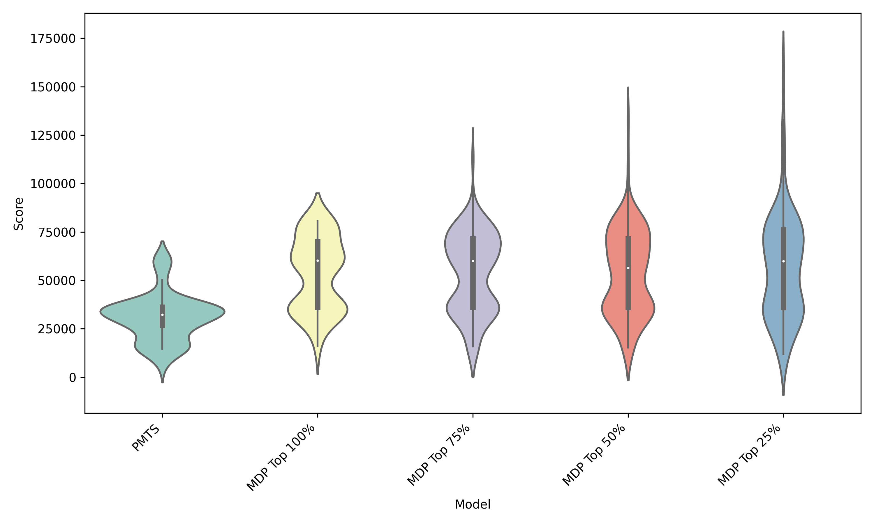
We can clearly see that using the MDP-formalized algorithm has better performance across the board compared to the pure Monte Carlo tree search. We can also see that selecting a subset of moves for the Monte Carlo evaluation is a high risk, high reward strategy. When not discarding any Monte Carlo games, the algorithm obtains the highest win-rate (2048 tile). As we discard more and more of the simulations, the win-rate goes down, but the rate at which the 8192 tile is reached increases. Reaching the 8192 tile requires merging 4 seperate 2048 tiles!
It makes sense that discarding more Monte Carlo simulations is high risk high reward, because each time a simulation is discarded, some information is lost. The simulations which are discarded are those with the lowest score, which implies that these simulations account for the worst case, or the most “adversarial” the tile spawns could be.
Discussion
Model score is most strongly influenced by the proportion of time the 4096 tile is reached. Many trials (with a wide range of parameters) which do not reach the 4096 tile achieve a score around 36,000, when they are near the 4096 tile. AI strategies are likely to fail shortly before reaching the next milestone tile because this is when there are the most high tiles on the board which can not yet be joined. Once reaching the 4096 tile, it is uncommon for a score below 60,000 to be reached, although there is a meaningful distribution between 60,000 and 80,000, where 80,000 represents the point near achieving a 8192 tile. This distribution of results requires that a given set of parameters is evaluated multiple times on the model before reporting performance. In order to illustrate this, consider the following example:
Suppose that a set of parameters $\vec{\theta_1}$ has a true probability of reaching the 4096 tile 60\% of the time, with the model scoring 35,000 when it doesn’t reach 4096, and 70,000 when it does. This means that a score of $56,000 = 0.6(70,000) + 0.4(35,000)$ should be reported as the long term expected performance of $\vec{\theta_1}$. If $\vec{\theta_1}$ is tested 3 times, the probability of 0.375 that the AI would report a score of 47,333 by reaching 4096 only once in the three runs. With 9 repeats, the probability of 47,333 or a worse score being reported (reaching 4096 3 times or fewer of 9) is 0.099. Running the parameters 9 times drastically reduces the noisiness of the data, which provides a much more accurate representation of parameter performance. This enables the Bayesian optimization model (as discussed in section 6.1) to make more accurate predictions about how future sets of parameters will perform.
Future directions
### Parameter optimization
As of the time of writing (summer 2023), this is an ongoing project, and the next thing I hope to implement is the optimization of $\vec{\theta}$, the parameter vector which controls how many random Monte Carlo searches to perform for a given number of empty tiles. The goal is to find the optimal tradeoff of time vs score. Below is a rough outline of the plan:
- Use a Quasi-Monte Carlo sampling technique with low discrepancy (such as Latin Hypercube Sampling or Sobol sampling) to draw a series of samples within the parameter space.
- Use Bayesian Optimization to determine which sets of parameters to evaluate next. (Implementation details such as Acquisition function not yet sorted out)
I intend to optimize for both move speed and score, and find the pareto efficient solution set which lets me choose the optimal speed and average score of the final model. Bayesian optimization is likely a strong framework for parameter optimization because it calls the target function (which can be non-differentiable) fewer times than other methods like evolutionary algorithms.
Dynamic policy switching
It is possible that when there are few tiles on the board, and explicit exploration of greater depth would be beneficial. Dynamically switching to an Expectimax algorithm seems like it may have strong results here. Expectimax uses Equation $\eqref{Bellman_policy}$ with a recursive value function given by Equation $\eqref{expectimax_value_fn}$.
Equation $\eqref{expectimax_value_fn}$ would evaluate to a certain recursive depth, and then call Algorithm 3 as the final evaulation of $V(s, \vec{\theta})$ to estimate the value at the final search state. This strategy would be particularly useful when there are few open tiles on the board because the low number of states to search increases the maximum search depth in a given amount of time.